In the last post I introduced the area of Frequent Subgraph Mining (FSM). As already mentioned there, one can use different metrics and algorithms to solve the different problems that occur in context of FSM. This post will now introduce a new algorithm for FSM on a single large graph. In contrast to other algorithms like GraMi [1], the here presented algorithm can be executed in parallel on a computer cluster and thus making it possible to also analyze very big graph datasets in an accetable amount of time.
The next sections will introduce the different steps of the so-called PaSiGraM (Parallel Single Graph Mining) algorithm. Therefor, I will first introduce the principle idea of PaSiGraM, before I dive deeper into the representation used for the single computations on the input and subgraphs. After that I will explain how PaSiGraM solves the steps of candidate generation and significance computation. Also some optimization techniques will be presented, to reduce the complexity of the algorithm further and thus making it more efficient. Last but not least the parallelization of the algorithms will also be discussed. At this point I want also to mention that the interested reader can also look at the code base of PaSiGraM at my GitHub repository. Currently the code is under development. The principle algorithm works but I want to add some extra functionality and also some more optimizations to further improve the perfomance of the overall algorithm.
Principle idea
Back to the logical structure of PaSiGraM. Like all other FSM algorithms, PaSiGraM is characterized by the substeps of candidate generation and significance computation. For that existing concepts were used. Examples are GraMi[1], FFSM[2] , FSG[3] or also SiGraM[4]. In general PaSiGraM explores the search space of all possible candidates according to the principle of breath first search. That means that candidate generation as well as significance computation are executed level-based.
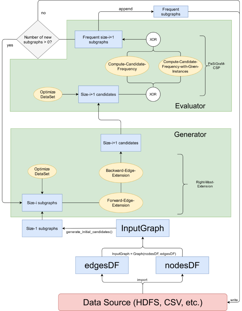
Figure 1 shows an example of the complete execution process of PaSigraM. The blue boxes represent the single data structures in which the corresponding graphs are stored. The functions of the algorithm are represented as yellow circles. Finally the two main components of PaSiGraM (Generator and Evaluator) are shown as green boxes in figure 1.
As we can see the algorithm starts with the import of the input graph. For this the edges and nodes will be load into different datasets. Both sets togehter then form our input graph, for which we want to compute the frequent edges as a first step. Based on this we can execute the candidate generation (named as Generator) and significance computation (named as Evaluator). The complete procedure wil be repeated as long as in the new iteration new frequent subgraphs will be found. At this point I refer back to the fact that PaSiGraM works level-based. This means that the whole procedure is executed for all subgraphs of size \(k\) before continuing with subgraphs of size \(k+1\).
A more detailed description of what happens in the two main components will be given in the further sections.
Graph representation
As already mentioned in the previous post, a graph can be represented by its adjacency matrix. This approach is also used for PaSigraM. The problem of this approach is, that we can generate several adjacency matrices (depending on the order of the nodes in the matrix) for a single graph. You can see an example for this in figure 2.
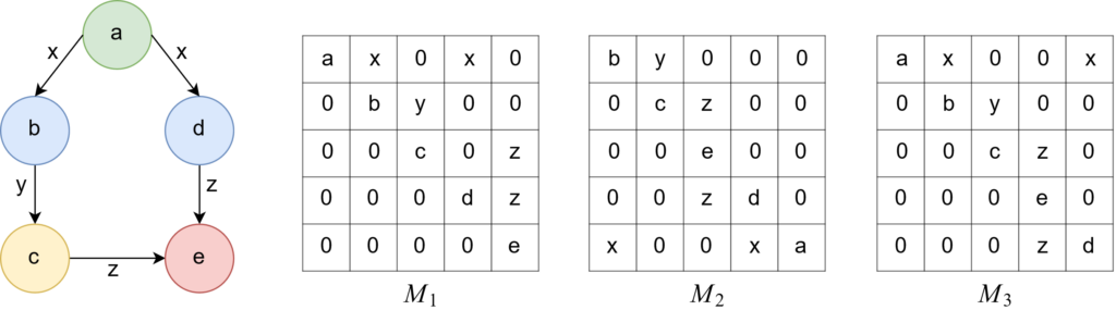
Because we generate the code of a graph by traversing its adjacency matrix from the top left to the bottom right, we would end up with different codes for the same graph.
For this reason the so-called CAM model (Canononical Adjacency Matrix) of Huan, W. Wang, and J. Prins[2] is introduced here. This model uses the lexicographically largest code for a graph, which is also called its canonical code. In this context it should also be mentioned that the same lexicographically largest code would be generated from the adjacency matrices of graphs that are isomorphic to each other. The adjacency matrix, which then leads to the canonical code of a graph, reffered to as CAM.
Definition 1 (Canonical Adjacency Matrix)
The CAM of a graph \(G\) is the adjcency matrix that produces the largest lexicographical code for \(G\).
In the example from figure 2 the adjacency matrix \(M_1\) would lead to the lexicographically largest code (\(M_1 :
ax0x00by0000c0z000dz0000e > M_2 : by0000cz0000e0000zd0x00xa > M_3 : ax00x0by0000cz0000e0000zd\)). Thus, we conclude that \(M_1\) is our CAM for this graph.
In PaSiGraM this idea is picked up but realized in a sligthly different way. Instead of using a matrix to generate the canonical code for a graph, we use a type of adjacency list. The model we use is reffered to as the CSP-list model. It is inspired by the CAM and characterized by the nodes, edges and the respective labels of a graph. But instead of using a marix, we use a list or table to represent the whole graph. An example for a CSP-list can be seen in figure 3.
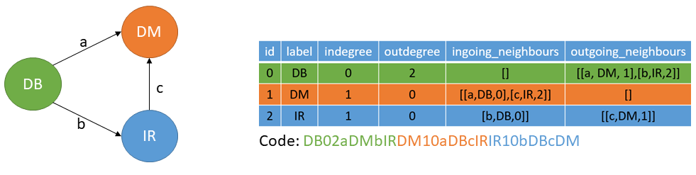
As it can be seen we collect a bunch of information for every node in the graph. The label column refers to the labels of the nodes. Indegree and outdegree each describing how many ongoing and outgoing edges the respective node has. The same applies for the in- and outgoing neighbours, with the difference that this columns consists of a list of lists. The entries of the encapusled lists are characterized by the edge label, label of the neighbour node and the ID of the neighbour node.
Out of the single rows of the CSP-list we can generate the unique code of a graph by combining the single entries for each row and sorting them according to its lexicographical order. In this contect it should also be mentioned, that the lists for ingoing and outgoing neighbours are also lexicographically ordered and that the IDs of the nodes are irgnored during the procedure of code generation.
Candidate generation
In order to shrink down the search space of all possible subgraphs/candidates, PaSiGraM also makes use of the anti-monotonic property (as it is defined in this post). In doing so the algorithm generates its candidates according to the pattern-growth approach. However, the number of possible candidates that can be generated from a graph can still be very large. To prevent this, PaSiGraM uses the so-called right-most-extension [4] to generate the next largest candidates from frequent subgraphs. In contrast to the conventional pattern-growth approach, an edge in the right-most-extension is not added randomly, but only at certain nodes. This means, that only nodes which are part of the right-most-path can be extended with a new edge.
Definition 2 (Right-most-path)
The right-most-path of a graph \(G\) is the shortest path from the root node (first added node) to the right-most-node (last added node). For the case of directed graph, the direction of the edges will be ignored to compute the right-most-path.
To extend the nodes in the right-most-path by a new edge, we use two different operations:
- Forward-edge-extension: Extends the graph by one edge which connects an existing node in the right-most-path with a new node (graph will be extended by a new edge and node).
- Backward-edge-extension: Extends the graph by one edge which connects the right-most-node to a node in the right-most-path (graph will be extended by a new edge).
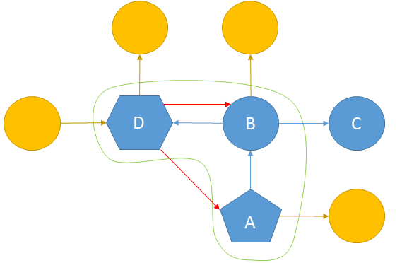
In figure 4 we can see an example for a right-most-extension of an existing graph. The yellow nodes are the nodes which could be extended by the forward-edge-extension (the green line marks all nodes of the right-most-path). The red edges could be added by backward-edge-extension (node \(D\) is the right-most-node and \(A\) is the root node). Node \(C\) is ignored, because it’s not part of the right-most-path here.
With this method we can shrink further reduce the search space of all possible candidates. This method is also the reason, why PaSiGraM computes all frequent edges at the very beginning of the whole procedure. Because due to the anti-monotonic property we just can add edges which meets the min support.
In this way, PaSiGraM can generate all possible candidates. If there are generated complete equal candidates, they can identified using their canonical codes which I already explained in the last section.
Significance computation
I already mentioned that a graph can be represented by its CAM. For the significance computation we use this fact as a basis to avoid the problem of subgraph isomorphism. To compute the frequency of a candidate, PaSiGraM uses a constraint satisfaction problem (CSP) in combination with the CAM of a graph.
Definition 3 (PaSiGraM-CSP)
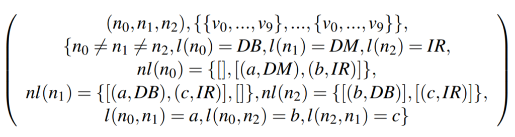
Let \(G_s = (V_s, E_s, l_s)\) be a subgraph of graph \(G = (V, E, l)\). \(l(v) \in L\) is the label of a node \(v \in V\) and \(l_s(v_s) \in L_s\) the label of a node \(v_s \in V_s\). Let \(nl(v) = {(l(e), nv)}\) be the adjacency list of a node \(v \in V\) and \(nl(v_s) = {(l(e_s), nv_s)}\) be the adjacency list of a node \(v_s \in V_s\), where \(l(e)\) or \(l_s(e_s)\) are the label of an edge \(e \in E, e_s \in E_s\) and \(nv\) or \(nv_s\) are the neighbor nodes, which are connected to \(v, v_s\) via the edges \(e\) or \(e_s\). Therefor the resulting \(CSP = (X, D, C)\) is defined as follows:
The variables are the nodes of the candidate and the domains of the variables are the nodes of the input graph. The solution of the PaSiGraM-CSP is then, to find valid assignments for each variable in its domain without violating the constraints in \(C\). Therefore, a valid assigment of a \(v_S\) to \(v\) is only given if they have the same label, if the neighbours of \(v_S\) are equal or a subset to the neighbours of \(v\) and if the labels of all ingoing and outgoing edges are the same.
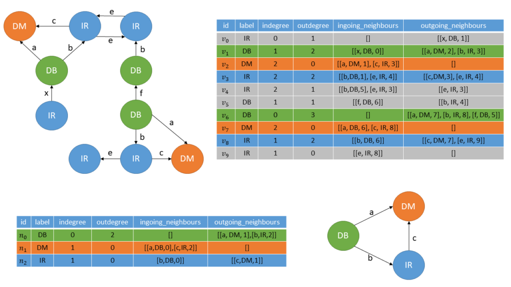
In figure 5 we can see an example for an input graph and a possible candidate. To compute the frequency of the candidate we have first to build the corresponding CSP:
When searching for a valid assignment for the node \(n_0\) of the candidate, we only have to take the nodes \(v_1, v_6\) into consideration, beacuse they have the same label and an in- and outdegree greater or equal to the one of \(n_0\). A valid assignment is found if all elements of the adjacency list of the node are found in the adjacency list of the respective node in the input graph. In figure 5 the valid assignments are marked by the colored lines in the adjacency lists of the respective nodes. The significance then corresponds to the smallest number of valid assignments of the nodes of the subgraph. For example the subgraph in figure 5 only has a significance of 2. This corresponds to the \textit{MNI} significance we already explained in the previous post.
Optimizations
PaSiGraM uses several optimizations to speedup the computation of the single steps. This section will outline some of these techniques.
Node decomposition. This technique describes the fact that the size of the domains for each variable of the PaSiGram-CSP can be reduced from the beginning. This reduction is given by the special properties of the CAM. Since the respective nodes are divided into clusters, we only have to obtain the clusters in the search process, which also contain nodes that have the same label and the same indegree as well as outdegree as the respective candidate node. Also the problem of automorphism is solved by this properties. An automorphism is an isomorphism of a graph to itself and appears because of symmetries in the respective graph. Nodes which are having the same adjacency lists and labels are treated as equal. Therefor they are stored as one node in the corresponding cluster, but are still marked as two different nodes in the respective graph.
Embedding transfer. Since we derive a new candidate from its respective parent graph by adding an edge to it, the resulting CSP problem can be reduced. The valid assignments for the nodes of the respective parent graph are passed to the new candidate. This eliminates the need to search for valid assignments for all nodes of the candidate. Instead, the assignments of all candidate nodes that are not involved in the newly inserted edge can be copied from its parent graph. This means that we only have to solve the resulting CSP problem for the two candidate nodes that are connected by the newly inserted edge. If both nodes have already been included in the parent graph, we only have to consider the nodes which are already included as valid assignments of the respective parent graph. This leads to the fact that the resulting CSP has to be solved only for the nodes which are connected by the newly inserted edge and not for all nodes of the respective candidate.
Load balancing. Between the two substeps candidate generation and significance computation, the new candidates must always be sent to the respective other procedure and the data record that contains the candidates must therefore always be distributed anew to the different nodes of a cluster so that the two substeps can each be calculated in parallel. This can lead to the following problem: The data record is distributed unevenly. As a result, some nodes in the cluster require more time to generate candidates or calculate significance. Since each of the two substeps of PaSiGraM (significance calculation, candidate generation) can only be executed once the previous substep has been completely scheduled, this would slow down the algorithm. In order to avoid this problem, PaSiGraM makes sure that the respective data sets are evenly distributed between the cluster nodes. During candidate generation, the frequent subgraphs of the last iteration step are divided in such a way that each cluster node has the same number of subgraphs from which it can then generate the new candidates. In the significance computation, the set of newly created candidates is also divided among the respective cluster nodes.
Implementation
As a basis I used Python as the programming language to implement PaSiGraM, because of its popularity for machine learning applications and the increasing interest in this language. The complete project is structured in three main Python packages: controller, model and services. The model package consists of all necessary data structures, such as a Graph, Edges and Nodes class. The different classes, which are all implemented as Python objects contain several attributes, which also can be implemented in extra classes. To speedup the calculation on single data structures, we use for them DataFrames. This data structure allows us to perform fast SQL like queries on a huge amount of data. Example queries could be grouping, selecting single entries and also concatenating two different data sets with each other. In addition, the calculations on the DataFrames can be distributed over several cores, which should mean an additional speedup.
The controller package includes the interface of the algorithm, as well as different classes for the generation and frequency calculation steps of PaSiGraM. The service package consists of different files which implements the functionality of the different classes. This is designed to separate the structure of the classes from their functionality.
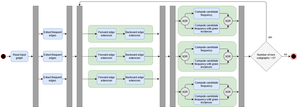
To parallelize the single computation steps of PaSiGraM, Iused Apache Spark. This framework allows to distribute the computation over different nodes in a computer cluster. Therefor every cluster consists of a minimum of one NameNode, which manages the parallelization, and several worker nodes which execute the single computations. Spark comes with different libraries and APIs such as GraphX, SparkSQL, SparkStreaming and the RDD API. For our purpose we just need the RDD API, which includes a data structure called Resilient Distributed Data Sets (RDD). With this API we can perform different operations on the given RDDs, which can contain for example Python objects. Therefore we are saving the single graph objects in such a RDD to parallelize the single computation steps of PaSiGraM. Spark then organizes aspects such as parallel calculation and fault tolerance for us. In figure 6 you can see the parallel execution of the PaSiGraM algorithm. The grey boxes are the splitting or joining of a parallelization step. As already mentioned PaSiGraM distributes the data sets of the candidates by itself. For that, we use the possibility given by Spark to partition the RDDs manually.
The code for the whole project can be found here at my GitHub page. Just for notice: The algorithm is currently under construction so basic functionality works but I plan to implement further optimizations to make the overall algorithm faster and more efficient int terms of used memory.
Citation
If you want to cite this article, please do it in the following way:
Ole Fenske, "PaSiGraM - an algorithm for FSM on a single graph". https://ole-fenske.de/?p=898, 2020.You can also use the bitex format if you are writing in LaTex:
@misc{fenske2020pasigram,
author = {Fenske, Ole},
title = {{PaSiGraM - an algorithm for FSM on a single graph}},
year = {2020},
howpublished = {\url{https://ole-fenske.de/?p=898}},
}
Literature
- [1]M. Elseidy, E. Abdelhamid, S. Skiadopoulos, and P. Kalnis, “GraMi,” Proc. VLDB Endow., pp. 517–528, Mar. 2014, doi: 10.14778/2732286.2732289.
- [2]J. Huan, W. Wang, and J. Prins, “Efficient mining of frequent subgraphs in the presence of isomorphism,” presented at the Third IEEE International Conference on Data Mining, 2003, doi: 10.1109/icdm.2003.1250974.
- [3]M. Kuramochi and G. Karypis, “An efficient algorithm for discovering frequent subgraphs,” IEEE Trans. Knowl. Data Eng., pp. 1038–1051, Sep. 2004, doi: 10.1109/tkde.2004.33.
- [4]M. Kuramochi and G. Karypis, “Finding Frequent Patterns in a Large Sparse Graph*,” Data Mining and Knowledge Discovery, vol. 11, pp. 243–271, 2005.